The blog was down for just over a week, the machine hosting it just suddenly refused to post. This was one month after the three-year warranty ran out, but Asrock came through and replaced it anyway, probably because there is a known hardware problem on these low-power “Avoton” boards.
Anyway, I’ve done a lot more NC30 tuning and had to change my strategy a couple of times, so I thought I’d give an update.
One thing that’s been kind of helpful is to record audio along with the Megasquirt log. By syncing up the audio with the log it’s easier to remember what was happening, and since I was encountering occasional knocking that’s audible on the recording you can match up that with the log and see what the parameters are. Much easier and safer than trying to look at the cellphone doing the logging while riding around…
I’m using a Zoom H1 digital recorder and an external microphone stuffed into a sock on the dash. The sound is surprisingly good even at higher speeds, although it makes you appreciate how much louder the bike is at full throttle because I’ve yet to manage to not clip the sound level. Here’s a proof of concept, just riding around a bit:
As you can see, the logs contain an absolute load of information. The four panes I plotted in the movie are as follows:
Top pane, main fueling variables:
- White: RPM.
- Red: manifold pressure as percentage of atmospheric pressure.
- Green: throttle position in percent.
Second pane: Air/fuel ratio:
- White, red: rear and front cylinder pair air/fuel ratios (AFR), expressed as lambda offset from the target lambda. This means positive values are leaner than desired, negative values richer. The values have the exhaust gas correction “undone” from them, so they’re not actually what the AFR was, it’s what it would have been if the correction had been disabled.
- Green, yellow: exhaust gas correction factors, as percentages, for the rear and front cylinder pairs. Since the tune isn’t perfect, the AFR won’t be exactly right. The controller will see this and attempt to “correct” by adding or removing fuel. This makes it less likely the engine will run lean because of a bad tune, which can lead to knocking. The controller is only allowed to add/subtract 15%.
Third pane: Temperature-related variables:
- Red: air density temperature correction, as a percentage of the density at standard temperature. The controller computes how much air the engine is pumping, and the warmer the air is, the less dense it is. This affects the calculation of how much fuel should be injected.
- Green: coolant temperature, in C.
- Yellow: manifold air temperature, in C.
Bottom pane: Volumetric efficiency
- White, red: computed volumetric efficiencies for the rear and front cylinder pairs. These come from the VE tables described in the previous tuning post.
So, with all that information, what’s the problem?
There’s been two things in particular that has been tricky to get right.
The first issue is the air density. There are two measurements of temperature, the air temperature in the intake and the coolant temperature, which basically is the temperature of the metal of the intake tract and the valve that the air passes through on its way into the cylinder. The effective temperature of the air, that determines the density of the air in the cylinders, will be somewhere between these two values. At full throttle the air flow is high and there’s less time for the air to change temperature from its temperature in the airbox, while at cruise power the air flow is less and the air will heat up more.
To take this effect into account, the engine controller uses a weighted average of the two temperatures when it calculates air density, where the weight is a function of the airflow through the engine. The trick is to figure out what this function should look like. To a large extent, this function is degenerate with the VE table, because a change is the calculated air density can be offset by a change in the volumetric efficiency.
The general idea is that this function starts out at 100%, which means the air temperature is equal to the coolant temperature, at very low airflow and then decreasing to reach 0%, which means the air density is only determined by the temperature of the incoming air, at some high airflow. But what’s the shape and how fast does it decrease?
The way I attempted to determine this was by looking at how the AFR changed as the bike warmed up. Since the amount of fuel being injected at a specific RPM and throttle position is always the same except for the air density correction, any change in air/fuel ratio as the motor warms up must be due to the temperature average being incorrect. If the engine runs leaner as it warms up, the engine is using too much coolant temperature in the average, leading it to calculate a too low air density and inject too little air. Conversely, if the engine gets richer as it warms up, it’s injecting too much fuel, meaning it’s overestimating the air density and thus underestimating how much the air warms up.
Here’s a plot of some of the data I gathered:
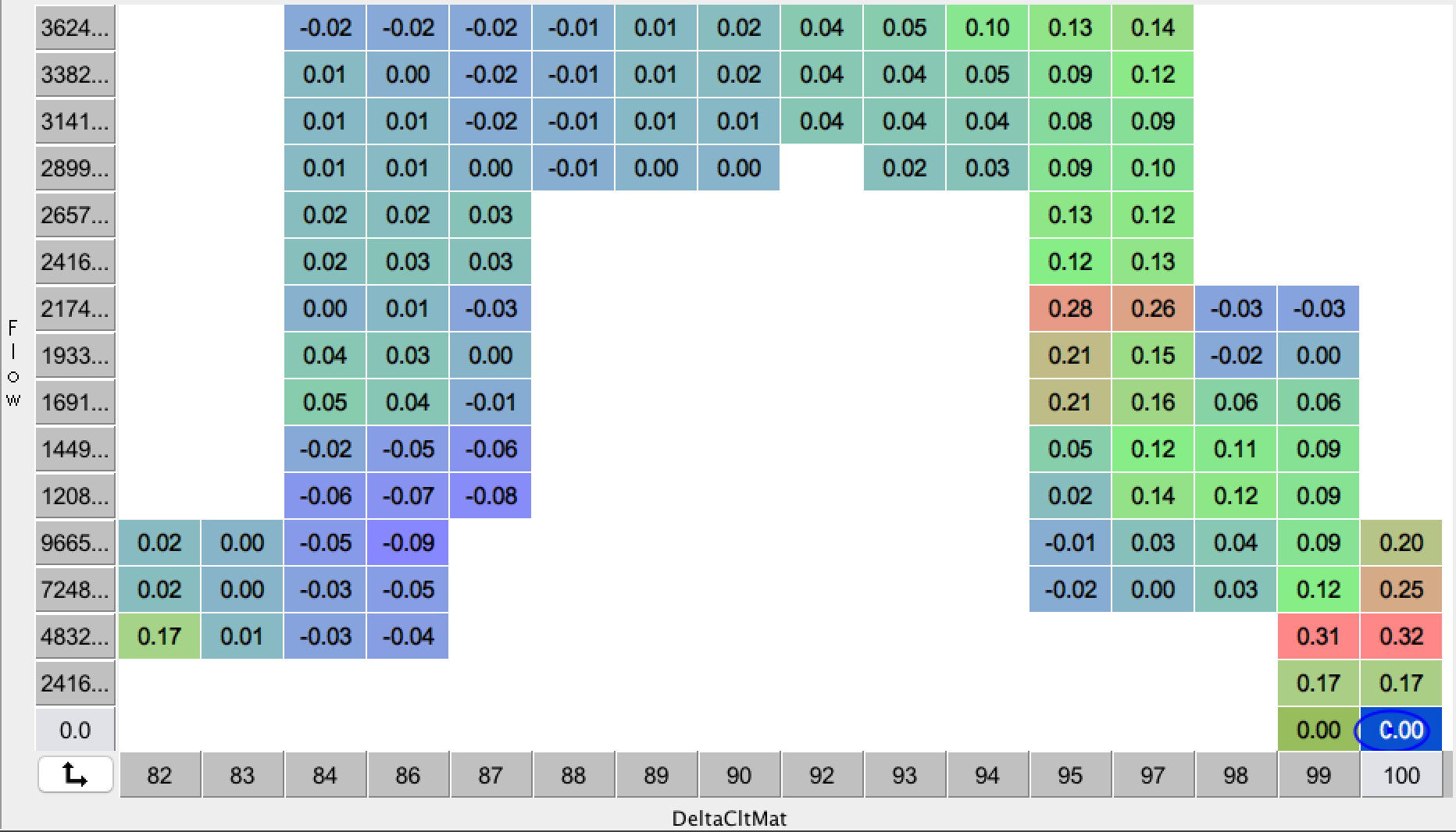
Data from a warmup run showing how the air/fuel ratio changes as the engine warm up. The X-axis is the air density at the coolant temperature as a percentage of the air density at the manifold air temperature. 100 means they are at the same temperature, i.e., the engine is cold. The Y-axis is airflow, calculated as RPM*manifold pressure.
Each box shows the air/fuel ratio offset from what’s desired. Positive numbers are lean.
If we look at the results across the higher airflows across the top, this is basically riding at roughly constant RPM and throttle. As the engine warms up, it moves to the left. The numbers across the top get smaller from the right to the left. This means the engine got richer as it warmed up, which means the ECU thought the air warmed up less than it really did.
In this case the engine got richer as it warmed up, so the air warmed up more than the ECU calculation assumed, and it overestimated the mass of air going in to the engine. (Strictly speaking, it’s not important here whether it’s over- or underestimated. The important conclusion is that it is more overestimated at high engine temperatures than at low ones.) This means the weighted average needs to have more coolant temperature and less manifold air temperature, at this airflow.
In practice, this effect is visible but quite subtle. It’s difficult to measure it at many different operating points, so it would be useful to have some theoretical expectation for what the shape of the curve should be.
If we make a simple Newtonian heat transfer model, which says that the heat flux between two materials of different temperatures T1 and T2 will be some constant k*(T1-T2). This in turn means material 1 will change temperature as a result of the energy flow as dT1/dt = -k*(T1-T2)/C, where C is the specific heat of the material.
This is a first order ODE that we can easily solve for the temperature difference, ΔT = T1-T2, and get
ΔT(t) =ΔT0 * exp(-k/C*t)
where ΔT0 is the initial temperature difference. This means that, in our case, the temperature of the air will exponentially approach the temperature of the intake.
Furthermore, for a given airflow F, it will take the air approximately a time t=V/F, where V is the volume of the intake, to pass through the intake tract. This is how long the air has to heat up. If we substitute this value for t into the expression above, we get
ΔT/ΔT0 = exp(-constant/F)
So this is the expected shape of the curve. As expected, for small F ΔT will approach zero, ie the air approaches the temperature of the engine, and at large F ΔT approaches ΔT0, ie the air has no time to change temperature at all.
In the context of our function, however, it is more convenient to talk about the percentage by which the air warms up, which is 1-ΔT/ΔT0. If the air doesn’t warm up at all, ΔT=ΔT0 and the percentage is zero. If we plot this function, it looks like this:
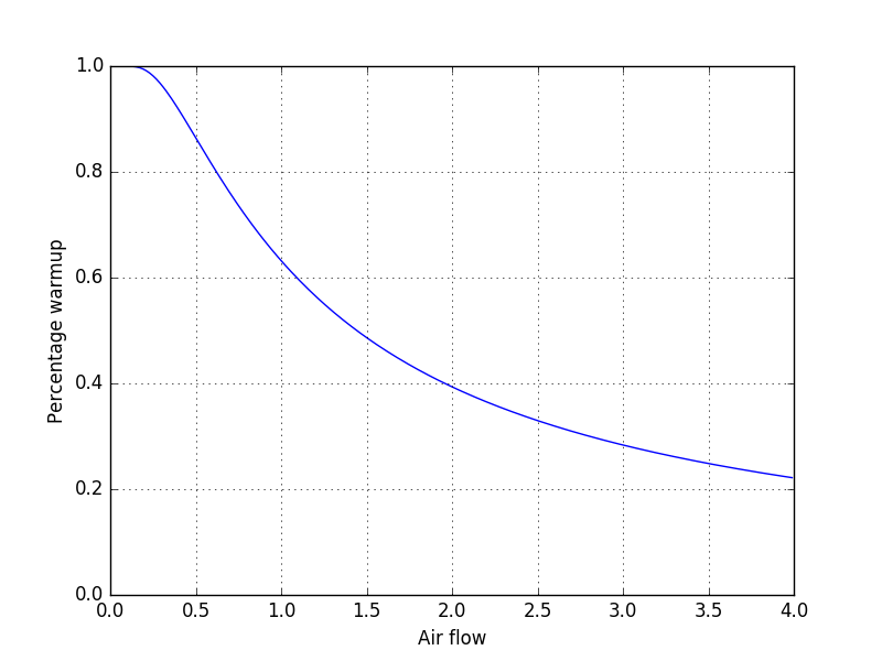
The theoretical expectation for how much the air will heat up towards the coolant temperature as a function of airflow. As you can see, for low flow rates the temperature fully reaches the coolant temperature, as expected. The curve declines quite slowly, however, so even for quite large flow rates there’s still an appreciable amount of heating. (The air flow scaling here is arbitrary.)
With this curve as a guide it would in principle be enough to have one point to be able to nail it down. I attempted to measure the effect at two airflows, at idle, which is near the “knee” in the curve where it dips downward, and at cruise power (the table shown earlier.) From these two points it was clear that the curve did not have exactly this shape, it actually appears to decline even slower than the curve would indicate (ie, the air heats up more). This is a much slower variation than I had initially thought it would be.
If you look at the “air density” in the movie log above, you can see that it quickly changes between two distinct values. These are the “air doesn’t heat up at all” and “air heats up all the way to the engine temp” cases, because I had a curve that quite quickly declined from 100% at near idle to 0% at just a bit higher air flows. With the new curve, the effect is much more gradual.
After refining these measurements on a couple of warmup runs, I think I have this part dialed in pretty well. There’s no longer a noticeable effect of the engine going leaner or richer as the temperature changes.
Well, that was the first tricky thing. However, this has already run on for longer than I thought, so I think I will save the second one for the next post.
Pingback: Microsquirting the NC30, part #46: Tricky Tuning – Patrik's projects